Today a quick tip that helped me out of a tight spot during one of my projects. The issue was that I received an Excel file with multiple PivotTables, but no source tables on which these PivotTables were built (these were in separate worksheets that were not shared). I needed the source data to produce my own custom complex reports (for which I use MS Queries instead of PivotTables), and I needed it now. Fortunately, PivotTables contain embedded source tables and there is a quick and easy way to recover Pivot Table data. Read on to learn how… maybe it will come useful.
How to reverse engineer a PivotTable
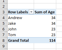
Let’s assume we have the following Excel PivotTable below.
Scroll to bottom right cell of the Pivot
In order to recover the Pivot Table data associated with the PivotTable you need to scroll down to the right-most, bottom-mostGrand Total value in the PivotTable.
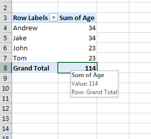
Double click on the Pivot cell
Now simply double-click on the Grand Total and the source table will appear on a separate Excel Worksheet as show below:
Easy right? Hope this helps you in similar situations – if yes, I appreciate a comment below!
O. M. G. It’s really that simple! Thanks 🙂 It appears that it doesn’t matter how many columns you have or whether you have anything in the Values area, just add a Grand Total row and double-click on the right-most cell in that row! Oh BTW, “Scroll to botton right …” is a typo …
Thanks for pointing out the typo. Yes that simple – good to remember it – especially when sharing PivotTables with other people when not wanting to share underlying data ;).


O. M. G. It’s really that simple! Thanks 🙂
It appears that it doesn’t matter how many columns you have or whether you have anything in the Values area, just add a Grand Total row and double-click on the right-most cell in that row!
Oh BTW, “Scroll to botton right …” is a typo …
Thanks for pointing out the typo.
Yes that simple – good to remember it – especially when sharing PivotTables with other people when not wanting to share underlying data ;).