Today something much lighter than usual, more to do with presenting data than just crunching it – How to Create an Excel Pictograph? Or, in other simpler words, How to Create an Excel Chart with Images!
Images are Powerful Stuff! Our Brain processes Images 60 Thousand Times Faster than Text! For us Consultants, Marketers and Office Clerks this is important to understand, although often neglected. Hence the term Death by PowerPoint, known also as Death By Slide – as in overwhelming your audience with an abundance of text and information squeezed into a single slide.
If you want to get Your Message across use Pictures instead. Today I will show you a simple, but effective Excel Trick you can use to make the most out of your Data Visualizations – to transform Dull Charts into Impressive Infographics.
How to Create an Excel Pictograph?
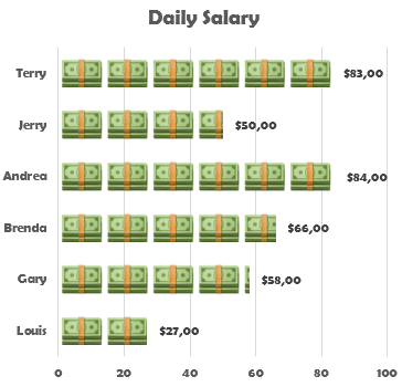 Let’s start with the Basics. An Excel Pictograph is a Chart that replaces standard Bars, Pies and other Graphic Elements with Pictures. Creating Excel Pictographs is incredibly easy, hence making it an incredibly Powerful Excel Tip / Trick.
Create an Excel Chart
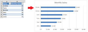
To create an Excel Pictograph we need to have a Chart to work on first. If you are new to Excel Charts feel free to listen to Chandoo’s Excel Chart Tutorial here. I created a simple Chart below:
Find an Image Icon for the Chart
The Chart above is Boring. Isn’t it? Just Raw Data. It takes a moment to take it in. Now let’s find an interesting image to replace the Boring Barchart! Here are some great resources I use to find Image Icons:
-
IconFinder a great database of Free and Premium Image Icons. I really appreciate the large amount of free images they have you don’t need to link back to
-
Icon Archive a clipart image database
-
Icon Finder yet another icon database
Be sure to find an Icon that will suitably visual the data you are trying to exemplify.
Paste the Image to your Excel Spreadsheet
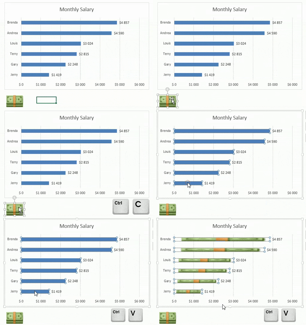
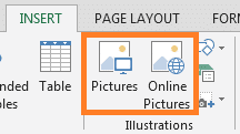 Now copy your image to your Excel Worksheet. To do that go to the INSERT Ribbon Excel tab. Select Pictures if you have the Image on your workstation, or Online Pictures if you need to download the Image from the Web. Follow the steps and hit Insert.
Copy & Paste the Image onto your Chart
-
Copy the Image by clicking on it and hitting CTRL+C
-
Select the Data Visual select your Charts Bars, Pie slices or any other Data Visual Element which you want to replace with an Image
-
Paste the Image by hitting CTRL+V
Configure the Image
The Chart is starting to look good. But often stretching the Image distorts it. We need to replace the Stretch with either the Stack or Stack and Scale with options:

-
Go to Data Series options by right clicking on the Bars and clicking Format Data Series...
-
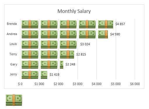
Go to Fill Options and select Stretch, Stack or Stack and Stretch with. That last options requires you specify the Units/Pictures ration. In our case 1000$ should equal to 1 picture, so I input 1000
Too make the Image look even better, you may also want to go to SERIES OPTIONS and adjust the Gap Width!
The Final Effect looks more like this:
