Often we need to merge worksheets / workbooks containing lots of data. Imagine receiving periodical daily reports and wanting to quickly consolidate them to generate a weekly or monthly report… seems like a lot of work. Merging worksheets does not necessarily need to be hard… as long as you read through today’s post.
Merging worksheets with VBA
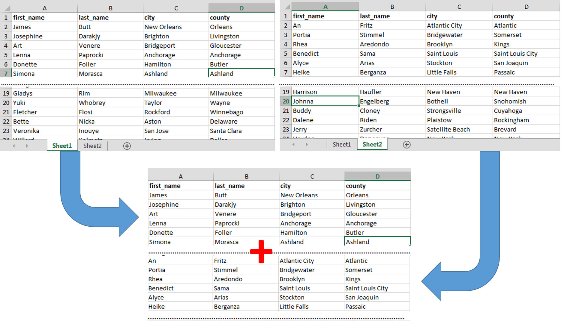
To exemplify the issue let’s consider a Workbook consisting of 2 worksheets (below named Sheet1 and Sheet2) with identical columns.

What we want to do is merge these 2 worksheets into one consolidated worksheet. We may of course want to do this in multiple ways e.g. by:
- Simply appending the worksheets to each other
- Merging the data sets while removing duplicates
Here is the example result we want to achieve (Sheet2 appended to Sheet1 on a third separate Worksheet):
In today’s Tip of the Day I will exemplify how to merge worksheets / tables (any number) with an option of eliminating duplicates.
Merging worksheets with VBA
Let’s first consider a simple piece of VBA code. The procedure below can handle any number of Worksheets – including Worksheets from external Workbooks as long as you have the Workbook open and provide it within the array of Worksheets passed to the procedure.
Sub Merge(ws() As Worksheet, destWs As Worksheet, headerInFirstRow As Boolean, removeDuplicates As Boolean)
    'Clear destination worksheet
    destWs.UsedRange.EntireRow.Delete
    Dim pasteRange As Range, header As Range, firstFreeRow As Range, w As Variant, copyRange As Range
    'Paste header
    If headerInFirstRow Then
        Set header = ws(0).UsedRange.Cells(1).EntireRow:
        header.Copy destWs.Cells(1).EntireRow
    End If
    Set firstFreeRow = destWs.UsedRange.Rows(destWs.UsedRange.Rows.Count).Offset(1).EntireRow
    'Paste worksheets
    For Each w In ws
        Set copyRange = w.UsedRange.Rows("" & _
            IIf(headerInFirstRow, 2, 1) & ":" & w.UsedRange.Rows.Count)
        copyRange.Copy firstFreeRow.Cells(1, 1)
        Set copyRange = Nothing
        Set firstFreeRow = destWs.UsedRange.Rows(destWs.UsedRange.Rows.Count).Offset(1).EntireRow
    Next w
    'Remove duplicates
    If removeDuplicates Then
        Dim colArr As Variant, col As Long: ReDim colArr(0 To destWs.UsedRange.Columns.Count - 1)
        For col = 1 To destWs.UsedRange.Columns.Count
            colArr(col - 1) = col
        Next col
        destWs.UsedRange.removeDuplicates Columns:=(colArr), header:=IIf(headerInFirstRow, xlYes, xlNo)
    End If
    'Clean
    Set firstFreeRow = Nothing: Set w = Nothing: Set header = Nothing
End Sub
A now a simple example of this procedure being used assuming the example data I referenced above. Let’s assume data on is on worksheets Sheet1 and Sheet2, the destination Worksheet will be Sheet3.
Sub TestMerge()
    Dim ws(0 To 1) As Worksheet
    Set ws(0) = Sheet1
    Set ws(1) = Sheet2
    Merge ws, Sheet3, True, False
End Sub
Notice that the Merge procedure accepts the following parameters:
- ws – an array of Worksheets
- destWs – the destination Worksheet
- headerInFirstRow – if true assumes that the header is in the first row of each source Worksheet
- removeDuplicates – if true remove all duplicates after merging the Worksheets
Simple enough right? Not too long. If you want to optimize it for best performance read this.
Merging worksheets with MS Query (SQL)
Now let’s consider a second approach – using MS Query (SQL). This is my personal favorite as MS Query SQL code is short, does not require VBA and the destination Worksheet can be refresh by simply right clicking on the table and hitting refresh.
To create a MS Query feel free to use my Excel SQL AddIn or follow the steps below:
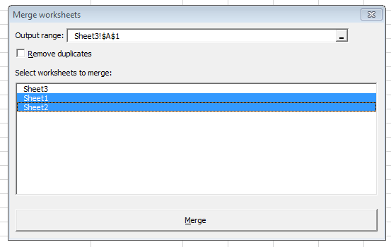
Follow the instructions below if you don’t have my Excel SQL AddIn:
Open the From Microsoft Query Wizard
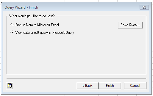
Data ribbon and then selecting From Other Sources and From Microsoft Query -> till the end be sure to hit View Data or Edit Query in Microsoft Query to be able to provide your own SQL query.
Proceed according to Wizard to edit SQL Query
As we want to merge several Worksheets within our current Excel Workbook we need to select Excel Files as the designated data source for our MS Query:

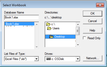
Next we need to select our Current Excel Workbook from the File Dialog:
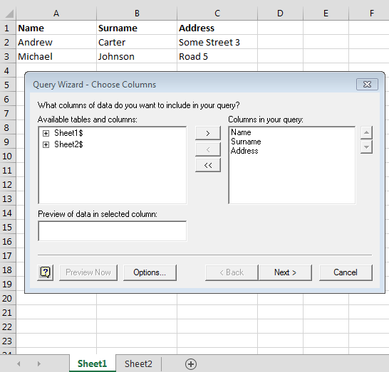
Select the first Excel Worksheet you want to merge and click the right arrow > to drag it to the Columns in your Query section.
Next instead of Returning the Data hit the View data or edit Query in Microsoft Query radio button and proceed:
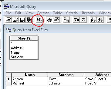
A new Window should pop-up. Look for the SQL button to modify the existing MS Query:
Modify the SQL Query to merge Worksheets
A new SQL Window should pop-up. You can modify any number of Worksheets using this approach. Below I am assuming I want to merge two Worksheets – Sheet1 and Sheet2. The MS Query need to therefore look like this:
SELECT * FROM [Sheet1$] UNION ALL SELECT * FROM [Sheet2$]
Simply modify the existing MS Query in the SQL Window and hit OK.
What if you need to merge 3 Worksheets not just 1?
Simply append an additional UNION ALL like this:
SELECT * FROM [Sheet1$] UNION ALL SELECT * FROM [Sheet2$] UNION ALL SELECT * FROM [Sheet3$]
For additional Worksheets repeat this pattern
Return Data to selected Worksheet
![]() Now the pleasant part – loading the Query data. Look for the Return Data button, select a cell where the MS Query is supposed to load and hit OK.
Now the pleasant part – loading the Query data. Look for the Return Data button, select a cell where the MS Query is supposed to load and hit OK.
Comment on using the MS Query approach
Simple and quick – this approach is more efficient than any VBA code we may develop as it is handled by the OLEDB driver. MS Query (SQL) is also more efficient in handling large chunks of data as compared to other approaches.
Merging worksheets with PowerQuery
If you are not familiar with PowerQuery feel free to download it from Microsoft here. PowerQuery features a lot of neat data-crunching / BI features. Let’s see how can we leverage PowerQuery to do our job.
Create tables from each source Worksheet
First what we need to do is link our source tables to PowerQuery so we can create the output query.

Select the whole range of each source worksheet (CTRL + A)
and select the From Table option from the
Merge the Worksheets
So now that we have our Tables configured in PowerQuery we can append the 2 (or more). Hit the Append button from the Combine group in the PowerQuery ribbon.

Next select Table1 from the first drop-down and Table2 from the second drop-down:
and hit OK
That’s it! Similarly as with the MS Query example you can always easily refresh your query by right-clicking and hitting Refresh!
Summary
I hope you found these methods useful. On one last note I would like to share my thoughts on how these methods compare.
Personally I prefer to use MS Query (SQL) via my SQL AddIn. This sentiment may of course be partially as I used to work a lot with databases and am used to coding SQL. I know for most Excel users out there this is not the case. In such cases and if you only have a couple of Worksheets you need to merge on a regular basis I do suggest downloading the PowerQuery AddIn. It’s easy to use and also allows you to refresh your query easily. In all other scenarios feel free to use the VBA approach and simply customize your code to work best for you!
Let me know if you found this useful! And be sure to subscribe to more Tips on my Twitter or Facebook page!







This is exactly what I am looking for, but is there a way to do this without using coding, or if I do not have access to MS Query (SQL) via my SQL AddIn?
True, I wrote this in 2015. Nowadays I would probably need to add PowerQuery as another way of merging worksheets without coding.