Today I want to elaborate shortly on how to correctly and easily number rows in Excel by adding dynamic row numbers using simple formulas. Every neat data table in Excel should have a numbering column in place so that every row can be easily reference at least by the item number. One way of numbering rows is to simply input the numbers and drag them down. However, this is a static manner and the numbering will not refresh automatically if you change the places of any rows or add/delete rows. Here I want to introduce several easy ways to achieve nice and neat dynamic row numbering in Excel. Ok so let’s dive right into 3 methods for achieving nice dynamic row numbers in Excel.
Let’s say we want to dynamically number rows counting also every empty row in between i.e. if there is an empty row between the numbers we want the numbering to account for that an increase the index. I use this approach most often due to it’s simplicity. See the example below on how this works.
The formula is very simple:
=ROW()-ROW(A$1)
A$1 is simply the header of the column to guarantee we start numbering from 1. Easy and neat right?
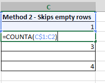
Method 2 – Dynamic numbering skipping empty rows
This time let’s account for every empty row in between. We want to continue the numbering from the last index. This comes in handy when you have sections of data or if you group the rows into different headers but want to retain the right numbering. See the example below:
Again the formula is dead simple:
=COUNTA(C$1:C1)
We use the static $ marker to make the range start from always the first cell in the column. The formula will count all non-blank rows so will skip any blanks we leave in between.
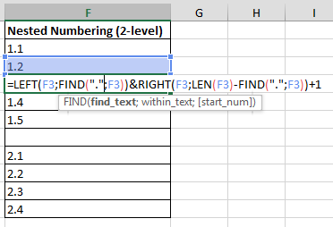
Dynamic nested numbering
Now for a bonus – dynamic nested numbering. Sometimes we need to add numbering with nested indices. I certainly encourage using nested numbering as it makes many tables more clear to read and the grouping more obvious. The approach/formula below can easily be reused to support nesting of additional levels. Numbering nested indices manually is often a nightmare if we need to frequently rearrange rows or add/delete some rows in between. Unfortunately, no formula will know for us when to automatically increment the first few nested indices (e.g. 1.2.1 to 1.3.1), but we can automatically increment the last index in the nested numbering index. See below.
We need to input manually add the first index e.g.
'Cell F2
1.1
Then below we can now use an automatic formula that we do the increment for us:
We can repeat this process with the next indices e.g. 2.1, 3.1 etc. We will always need to type the first one manually but the formula can help renumber the subsequent indices automatically e.g. 2.2,2.3,2.4 etc.
Hope this helps you with generating those dynamic row numbers!

 Today I want to elaborate shortly on how to correctly and easily number rows in Excel by adding dynamic row numbers using simple formulas. Every neat data table in Excel should have a numbering column in place so that every row can be easily reference at least by the item number. One way of numbering rows is to simply input the numbers and drag them down. However, this is a static manner and the numbering will not refresh automatically if you change the places of any rows or add/delete rows. Here I want to introduce several easy ways to achieve nice and neat dynamic row numbering in Excel. Ok so let’s dive right into 3 methods for achieving nice dynamic row numbers in Excel.
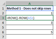


")