Cascading drop-down are a very useful feature in Excel making it much easier to categorize your records. Say you have a list of records you want to associate with categories and subcategories. Normally you would start by assigning a category to each record and then have a problem with matching a subcategory.
What is a cascading drop-down?
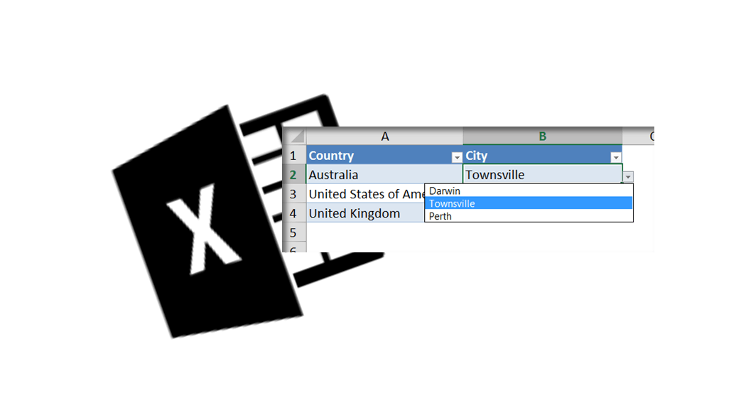
Cascading drop-downs are drop-downs that filter their values based on the selection made on another drop-down (higher in the hierarchy). You can have any amount of cascading drop-downs e.g. drill-down from store department, through the products lane, down till the product family and finally the product SKU. See the example below:
What to play with a online example? Telerik controls have a nice mock-up Cascading DropDownList for this.
How to make a cascading drop-down
Now down to business. Let’s go through the simple steps of creating a 1 level cascading drop-down consisting of 2 drop-downs. Simply repeat these steps to create additional cascading drop-downs levels.
Prepare source data for the drop-downs
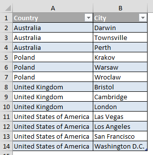
I prepared a simple data set consisting of countries and associated cities.
Notice that the countries are repeated for each city. This is because we need to map out each city with an individual country for what we are about to do in the next step. If you need to add an additional level for the cascading drop-down you should repeat this approach.
Create a named range for each category
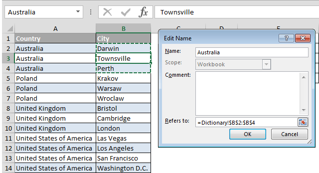
Create a named range for each country by selecting all cities within the country. Repeat this for all remaining countries. In case you need to add new subcategories (cities) to your cascading drop-down insert rows in the middle of a country section. This will automatically extend the named range.
Now for the the important part!!! Remember to name your countries using the exact name of the country. In case there are spaces in the names (which are not allowed in named ranges) replace them with “_”. This post handles such cases equally.
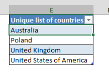
Create a unique list of unrepeating items for the first drop-down
You can either create this list manually or to just listing the countries manually for the first drop-down. I personally prefer to have the list created automatically based on the first column of countries in the examples above – use the formula below for that:
It’s best to use the same worksheet as the source tables and use the formula below to extract a unique repeating list of countries. This is an Array Formula so remember to hit CTRL+SHIFT+ENTER when editing the formula (first line only). Then simply drag/copy it down to get all countries.
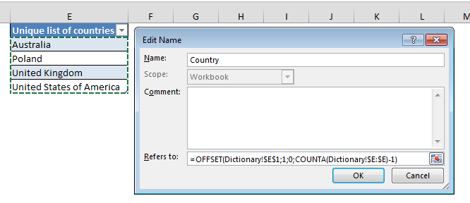
Array Formula for unique list of unrepeating countries
Assuming your list of countries is in column E of the same worksheet as shown above feel free to use the formula below for the named range – it will update the list automatically whenever you add new countries. Alternatively simply select the whole list of countries – but remember to update the named range manually when adding new countries.
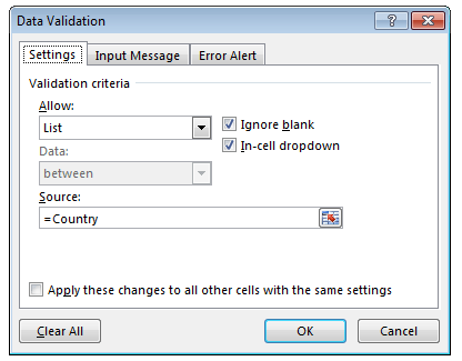
Create the cascading drop-down based on the named ranges using Data Validation
You are almost there! Now go to the worksheet where you want to define your cascading drop-down. And add Data Validation for the first and second cell as shown below:
First drop-down
Go to Data Validation and define the list based on the named range we created in Step 4:
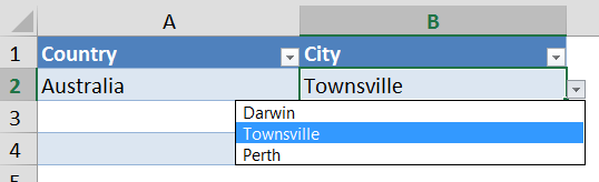
Second drop-down
Now let’s repeat the same exercise and again for the second cell we need to add Data Validation. This time we will use the INDIRECT function to dynamically associate the correct named range of cities based on the country selected in the first cell.